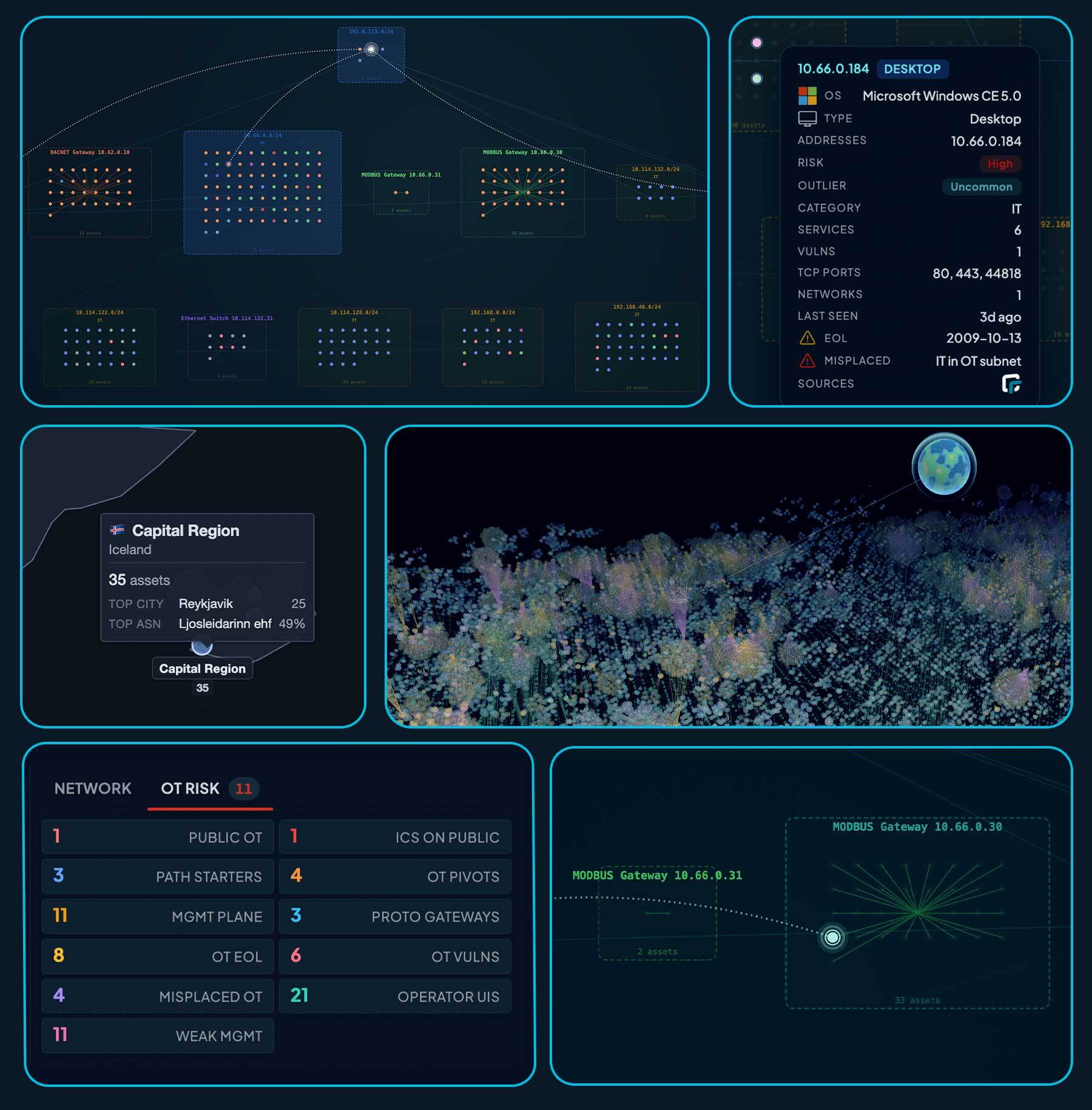
Network Map

Platform

The Network Map is an interactive Layer-2 / Layer-3 topology of every asset in the current scope. Where the World Map shows assets by physical location, the Network Map shows logical relationships: which subnets contain which assets, which gateways and switches connect them, and which assets pivot between subnets.

The map ships in two modes — a 2D Canvas view and a 3D rotating globe — that share the same data, search syntax, and trace engine.

Accessing the map

The Network Map can be opened from several places in the console:

• Inventory grid — Asset rows show a small map icon when the asset has L2/L3 data. Clicking the icon opens the map filtered to that asset.
• Inventory search — The “View on map” action above the inventory grid opens the map with the current inventory search applied as the map filter.
• Asset details — The Manage menu on an asset’s detail page offers View on network map (or Back to network map if you arrived from the map). The same menu also offers View internet attack path, which pre-loads a trace from the public internet to the selected asset.
• Reports — Open it directly at /reports/network/map from the Reports menu, or https://console.runzero.com/reports/network/map.
• Queries — Saved query rows in the queries grid include a “View on network map” action that prefills the map with the saved query.

When you open the map from another page, runZero records the previous URL as a return target. A Back button appears in the top-left and returns you to that exact view, preserving your filters and pagination.

2D and 3D modes

• 2D Network Map (/reports/network/map) — Canvas-rendered topology with the full feature set: hop-filter trace, choke-point analysis, multi-tab Network Intel card, search results panel, and rich exports.
• 3D Network Map (/reports/network/map/3d) — A rotating spherical layout that uses the same data, search syntax, and Source / Target trace engine. Useful for executive views and demos.

To switch modes, use the 2D / 3D button in the toolbar. Filter, search, and trace state are preserved across the switch.

Subnet layout

The map groups assets into rectangular subnet clusters. Each subnet box contains the assets that have at least one address in that CIDR range, along with any unaddressed (MAC-only) endpoints linked into the subnet by L2 evidence.

Subnet mask

The toolbar mask selector controls how IPv4 addresses are aggregated into subnets:

• /24 (default) — each /24 is a separate cluster.
• /16 — collapses related /24s into the same /16 parent.
• /15 through /8 — broader rollups, useful for large flat networks.

A separate selector controls the IPv6 mask, which defaults to /56 and ranges from /32 to /64 in steps of 4.

When runZero scans a subnet that overlaps with a configured site subnet, the configured CIDR is used directly. Otherwise the chosen mask is applied to the asset’s address to derive a synthetic subnet boundary.

Multi-homed assets

A single asset that has IP addresses in more than one subnet appears once in each subnet it belongs to. The renderer draws an L3 link between each copy so the map clearly shows the asset bridges those segments. The same asset ID is used for every copy — clicking any copy opens the same asset detail panel — but each copy has its own position so trace paths through the asset are visually unambiguous.

Multi-homed assets are counted as Pivots in the Network Intel card (multi_homed:t).

Public Internet node

A virtual Public Internet node is pinned at the top of the layout. Public IP subnets observed during scanning attach to this node, and the trace engine treats it as a valid source / target for ingress and egress path analysis (see Tracing paths).

By default the map filters out widely-reused public IPs (for example public DNS resolvers like 1.1.1.1 or 8.8.8.8) that show up on many internal assets and would otherwise produce misleading internet edges. The threshold is configurable in the Trace panel’s expanded view.

Network Intel card

The Network Intel card on the left rail is a clickable stats grid. Each cell shows a derived count for the current view; clicking a cell seeds the map’s search bar with the corresponding query and re-runs the filter.

Cell	What it counts	Click query
Assets	Total assets in view	(display only)
Subnets	Distinct subnets observed	(display only)
High Risk	Assets with high or critical risk	risk:high OR risk:critical
EOL	Assets running an end-of-life OS	eol:t
Pivots	Multi-homed assets bridging two or more subnets	multi_homed:t
Public	Assets with at least one public IP	has_public:t
Misplaced	Assets whose category does not match their subnet’s classification	misplaced:t
Outliers	Assets that are distinct from their neighbors’ norm	outlier_rank:>1
Gateways	Protocol gateways bridging IP and non-IP networks	gateway:t AND NOT gateway_kind:switch
Switches	Managed switches that share neighbor information	gateway_kind:switch

The card also includes a device-type legend; each legend cell is clickable and runs an equivalent type: or category: query.

OT Risk tab

When the current view contains OT-scoped assets, an OT Risk tab appears alongside Network. It is a curated grid of one-click investigations driven by the OT risk register. Each card runs a query against the visible map and shows the result count; click a card to filter the map and the inventory below.

Card	What it surfaces
Public OT	OT-scoped assets reachable from the public internet — ot_scope:t AND has_public:t
ICS on Public	Native ICS protocols (Modbus, EtherNet/IP, DNP3, BACnet, S7, OPC UA, IEC-104, KNX, …) on a public IP
Path Starters	Internet-facing management / lateral-movement services (RDP, SMB, SSH, WinRM, VNC, Telnet, VPN, IPMI)
OT Pivots	OT-scoped assets that are multi-homed across subnets — ot_scope:t AND multi_homed:t
Mgmt Plane	OT-scoped management-plane services (SSH, RDP, SMB, WinRM, VNC, Telnet, IPMI, BMC, KVM)
Proto Gateways	Protocol gateways bridging IP topology to BACnet, EtherNet/IP, Modbus, KNXnet/IP, C37.118, …
SIS Candidates	Hardware suggesting Safety Instrumented Systems (Triconex / HIMA / ProSafe)
OT EOL	OT-scoped assets on an end-of-life OS or firmware
OT Vulns	OT-scoped assets with high or critical risk
Misplaced OT	OT in a non-OT subnet, or non-OT in an OT subnet (segmentation gaps)
Operator UIs	OT-scoped HMIs, Panel PCs, engineering workstations, operator desktops, thin clients
Weak Mgmt	OT-scoped Telnet, FTP, VNC, TFTP, SNMPv1/v2c — cleartext or unauthenticated management

OT-scoping is computed from the asset’s category, the subnet classification, and a small device-type veto list (a Schneider UPS with a stale category:OT tag is not OT-scoped).

Search

The search bar accepts a domain-specific query language with keyword filters, free text, boolean operators (AND, OR, NOT), parentheses, and * wildcards. Bare text matches across all fields.

192.168.1                              # free-text match
name:web-server                        # keyword
type:server AND os:Linux               # boolean
NOT net:10.0.0.0/8                     # negation
(name:PC AND type:server) OR os:Windows
multi_homed:t AND has_public:t
type:Server AND geo:30.27,-97.74,25km

Identity, address, and platform

Keyword	Aliases	Matches
id		Node or asset ID
address	addr, addresses, ip, host	IP address(es)
name	names, hostname, hostnames	Hostname(s)
net	cidr	Subnet / network CIDR
type		Device type (Server, Desktop, Switch, IP Camera, …)
os		Operating system
os_version	osversion	OS version
hw	hardware	Hardware model
category	categories	Asset category (IT, OT, IoT)
subnet_class	net_class	Subnet classification (OT, IoT, General)
ot_scope		OT-scoped (t / f) — defers to category + subnet + vetoes
functions	function	Asset function tags
vendor	mac_vendor, newest_mac_vendor	Newest MAC vendor
tag	tags	Asset tags
domain	domains	DNS domains
site	site_name, site_id	Site
explorer	agent, last_agent_id	Last Explorer (UUID prefix)
task	last_task_id	Last task (UUID prefix)
detected_by	det	Detection method (arp, icmp, ndp, …)

Boolean / flag fields

Keyword	Matches
multi_homed	Asset has addresses in multiple subnets (t / f)
has_public	Asset has a public IP
has_private	Asset has a private IP
has_ipv4	Asset has at least one IPv4 address
has_ipv6	Asset has at least one IPv6 address
has_link_local	Asset has a link-local address
has_mac	Asset has MAC address data
has_os, has_hw, has_name, has_type	Asset has the named field populated
eol	Asset is end-of-life (t / f)
misplaced	Asset’s category does not match its subnet’s classification
unmapped_mac	Node is an unmapped-MAC stub from a switch port
gateway	t / f for any gateway, or a specific kind (see below)

Numeric fields

All numeric fields support comparisons (>, <, >=, <=, ranges).

Keyword	Matches
risk_rank	Numeric risk rank (0-4+)
outlier_rank	Outlier score rank (0-4+)
criticality	Criticality rank
modified_risk_rank	Modified risk rank (0 = unmodified)
vulnerability_count	Number of known vulnerabilities
software_count	Number of detected software packages
service_count	Number of detected services
mac_count	Number of MAC addresses
address_count	Number of IP addresses
name_count	Number of hostnames
service_ports_tcp	TCP port numbers (service_ports_tcp:443, service_ports_tcp:>1024)
service_ports_udp	UDP port numbers
rtt, lowest_rtt	Lowest round-trip time in microseconds
hops, ttl	Lowest TTL / hop count
newest_mac_age	Newest MAC age in seconds

Services and software

Keyword	Matches
service_protocols	Service protocols (http, ssh, tls, modbus, bacnet, …)
service_products	Service product names (Apache*, nginx, OpenSSH*)
protocol	Convenience alias for service_protocols
product	Convenience alias for service_products

Time

first_seen (alias firstseen) and last_seen (alias lastseen) accept relative ranges like <7days, >24hours, <30days, or absolute timestamps like >2026-01-01.

Risk

Keyword	Matches
risk	Risk level label (Critical, High, Medium, Low, None)

Node and gateway types

Keyword	Matches
node_type	Graph node type: a=asset, n=subnet, u=unaddressed, g=gateway, m=unmapped MAC, r=router hop
class	Object class: asset, subnet, gateway, unaddressed, unmapped-mac, router-hop, plus device-type aliases (switch, firewall, …)
gateway_kind	Gateway protocol kind: switch, bacnet, modbus, cip, knxnet, s7comm, dnp3, profinet, ethercat, omronfins, melsecq, hartip, c37118
switch_port	Switch port observation on an unmapped-MAC stub (e.g. Gi1/0/1)

Geographic search

Keyword	Aliases	Matches
geo	geo_within, geo_radius	Distance: geo:<lat>,<lon>[,<radius>] (km, mi, m, default 50km)
country		ISO country code
city		City
state	subdivision	State / subdivision
continent		Continent
postal_code	postal	Postal code
timezone		Timezone (America/Los_Angeles)
asn	isp	ASN ID or network owner
geo_source		Source of the geo point (isp, cloud-region, attribute-ip, …)

See Geolocation for how runZero produces these values.

Tracing paths

The Network map’s trace engine answers the question “how does traffic get from A to B?” by computing shortest paths through the rendered topology. The Trace panel at the top of the map controls every aspect of the trace.

Sources and targets

A trace needs at least one of:

• One or more Sources — the start of the path.
• One or more Targets — the end of the path.

You can supply sources and targets in three ways:

1. Right-click any node on the map and choose Add as Source or Add as Target.
2. Search, then assign — type a query into the search bar and click Set Query As Sources or Set Query As Targets in the trace panel. Every node matching the query becomes a source / target.
3. Open from asset details with the View internet attack path action — this pre-loads Public Internet as the source and the asset as the target.

The same selection methods work in 2D and 3D.

Trace modes

The button in the trace panel changes label based on what is set:

Sources set	Targets set	Mode label	Behavior
Yes	Yes	Trace Path	Shortest paths between every source and every target.
Yes	No	Trace Outbound	All paths reachable outward from the sources.
No	Yes	Trace Inbound	All paths converging on the targets from the rest of the graph.

Trace from the internet

To answer “what can reach this asset from the public internet?”, set Public Internet as the source (right-click the public internet node and choose Add as Source) and the asset of interest as the target, then click Trace Path. The asset details page View internet attack path action does this in one click.

To answer “what does this server expose to the internet?”, reverse it — set the asset as the source and Public Internet as the target.

IP version routing

The trace engine respects two IP-version toggles in the panel’s expanded view:

• Route IPv4 — include IPv4 paths in the trace (default on).
• Route IPv6 — include IPv6 paths in the trace (default on).

Two additional toggles control IPv6 visibility on the canvas itself, independent of routing:

• Show IPv6 link-local — render fe80::/10 addresses (default on).
• Show IPv6 global — render global unicast 2000::/3 addresses (default on).

Widely-reused public IP filter

By default the trace ignores public subnet nodes that are linked to more than 5 distinct internal assets. This filters out misleading edges introduced by shared resolvers (1.1.1.1, 8.8.8.8) and content-delivery anycast addresses. The threshold is configurable in the trace panel.

The Trace panel and per-hop filters

The collapsed trace panel shows the current Sources, Targets, and the trace button. Click the ▾ chevron to expand it and reveal the per-hop filter grid and the routing toggles described above.

Per-hop filters

The hop-filter grid lets you specify an exact attack path, hop by hop. Each row corresponds to one hop from the source and has two inputs:

• Include — only nodes matching this query may appear at this hop.
• Exclude — nodes matching this query are removed from this hop.

The inputs accept the full search query language described above, and the panel shows the live match count next to each input as you type.

These filters reduce any source → target paths to just the hops that satisfy the constraints. They are subtractive: they cannot add a path that doesn’t already exist in the graph, but they can carve a much smaller subset out of a noisy trace.

Examples:

• Force the path to pivot through SSH: put service_protocols:ssh in Hop 1 → Include.
• Exclude known firewalls and routers: put type:Firewall OR type:Router in Hop 1 → Exclude.
• Reach OT through a specific HMI: put type:HMI AND name:hmi-prod-* in Hop 2 → Include.
• Find paths that cross a multi-homed pivot: put multi_homed:t in Hop 1 → Include.
• Eliminate a specific subnet from consideration: put net:10.50.0.0/16 in any hop’s Exclude input.

Filters apply hop-by-hop counting from the source side. A trace with all four hop filters empty is the unconstrained shortest path; adding any include / exclude carves the result set without re-running the search server-side.

Choke points

When a trace produces results, a Choke Points panel appears on the left rail. It lists the assets that sit on the largest share of source → target paths — the systems that, if removed or hardened, would disrupt the most attack paths.

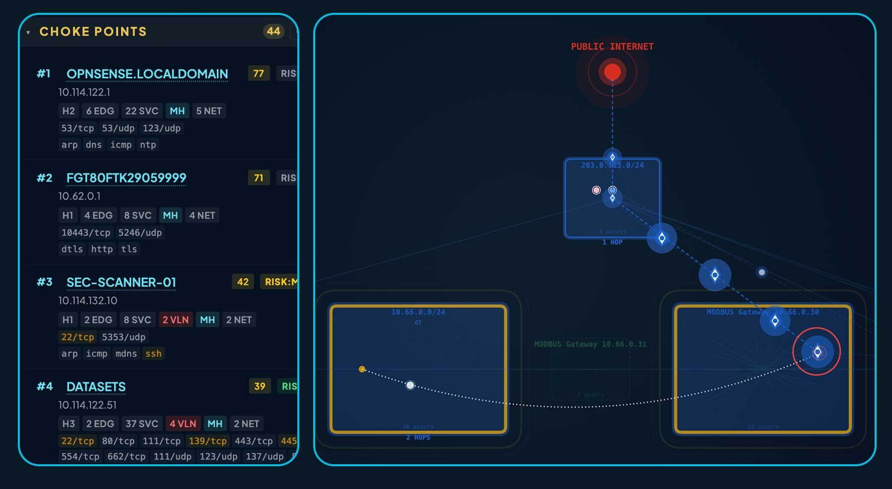
How choke points are scored

Each candidate is given a Pivot Risk Score that combines connectivity signals with a heavy bias toward devices that act as the only path into a non-IP backplane. Candidates are sorted by this score (descending), with ties broken by hop position and then by asset risk rank. The top of the list is what you should harden first.

The score is built from these signals:

Signal	Weight	Why it matters
Protocol-gateway pivot	+1000 (dominates the score)	A protocol gateway (BACnet, Modbus, EtherNet/IP CIP, KNXnet, S7, DNP3, …) is the only way to reach the assets on its backplane. Blocking it severs every downstream device, so it always ranks at the top.
Gateway pivot is also EOL or vulnerable	+200	Adds a “replace this first” boost when a protocol-gateway pivot is end-of-life or carries known vulnerabilities.
Cluster count (subnets bridged)	+15 per additional cluster beyond the first	Multi-homed assets that bridge two or more subnets concentrate transit traffic — each extra subnet they touch increases their leverage.
Edge count on the trace	+2 per edge, capped at 50 edges	Counts how many distinct neighbors the asset talks to on the trace path. Higher fan-in / fan-out means more flows pass through it.
Network count (distinct networks)	+5 per additional network beyond the first, capped at 10	Rewards bridging across separate networks (different CIDRs or routing domains) rather than just multiple subnets within the same network.
Multi-homed flag	+10 (one-time)	A small constant bump for any multi-homed asset, on top of the cluster / network counts above.
Service count	+1 per service, capped at 20	Heavily-exposed assets (many open services) are higher-value pivots than single-purpose hosts.

Candidates that do not meet a minimum bar are excluded from the panel entirely: an asset has to either bridge into a protocol gateway, have more than one neighbor on the trace, or be multi-homed across subnets. Protocol-gateway pivots are always kept regardless of degree because they are by construction the choke point for everything behind them. The list is capped at 100 entries so very large traces stay readable.

Reading the panel

Each row shows the priority number (1 = highest), the asset’s name and key attributes, and its Pivot Risk Score. Protocol-gateway rows are highlighted and include the gateway protocol kind plus the count of backplane assets that depend on it. Click a row to focus the asset on the canvas and reveal its full details.

The Show only protocol gateways toggle filters the list to gateway pivots, and the count badge in the section header still shows how many entries were hidden so you know whether more candidates exist. The full list — filtered or not — can be exported to CSV from the Export menu.

Exporting

The Export menu in the toolbar produces both image and graph-data formats from the current map view.

Images

• Current view (PNG) — exactly what is on screen, at the rendered resolution.
• Full network (PNG) — the whole topology rendered to a high-resolution PNG, regardless of the current pan and zoom.

The 3D map exports the current rotated view as PNG.

Graph data

These formats include nodes, edges, subnet clusters, and node positions, suitable for loading into other graph tools:

• GraphML — opens in Gephi, yEd, Cytoscape, NetworkX, and any GraphML-aware tool.
• GEXF — Gephi-native format with richer attribute typing than GraphML.
• GML — Cytoscape, R igraph, and other classic tools.
• Cytoscape JSON — direct import into Cytoscape Web and Cytoscape Desktop.
• Visio (VSDX) — opens in Microsoft Visio.

Tabular data

• Assets (CSV) — a flat asset table of the current view (or the search-filtered subset when a search is active).
• Choke Points (CSV) — one record per choke-point asset for the active trace.

Sharing a view

The map’s URL captures the current filter, pan / zoom, theme, mask, search query, and any active trace. Copy the browser URL — recipients with access to the same organization will see exactly the view you copied.